
An Alternative Way to Plot the Covariance Ellipse
An elegant and exact way to plot the confidence ellipse of a covariance.
Code, explanation, examples and proof.
Years ago, I was looking for a recipe to plot the confidence ellipse of a covariance. While working solutions where available, I had the idea that there should be a simpler and more elegant way. Shouldn’t we be able to plot the ellipse just using mean, standard deviation and the Pearson-Coefficient? This idea kept nagging for my attention and I managed to spend some time on it - on and off.
It looks so easy …
Intuitively, when looking at the means, standard deviations and the Pearson Correlation Coefficient of two variables, you can easily predict what the resulting ellipse will look like, but the methods that are circulated on the web - if they work at all - make you calculate eigenvalues explicitly and tweak angles, which seems like a lot of ado for such a “simple” task.
The best method and explanation I could find on the web is in an article by Vincent Spruyt. This one helped me out when I was in need of a quick solution.
However, I was not able to find anything on the web that resembles the simpler approach that I am describing here, so I think that it is worth sharing.
I found a way to plot the ellipse just using means, standard deviations and the Pearson Coefficient. I give explanations and a proof further down in this post, but here is the cookbook-recipe in case you are in a hurry (or happen to trust me blindly, which I discourage).
It is tempting to shout: “No eigenvalues involved”. But in fact, this is all about eigenvalues - we just do not have to calculate them as usual.
The Short Answer Is …
-
Calculate the covariance of the two variables x and y (or features or columns, whatever you call them). I assume that x will be plotted along the horizontal axis and y along the vertical axis.
-
Normalize the covariance by dividing it by the product of the standard deviations of the variables. This yields the Pearson Correlation Coefficient ($p$)
- Use your plotting framework to draw an ellipse that is centered at the origin, its axes aligned with the axes of the coordinate system. The ellipse has the following radii (not diameters!)
-
Rotate the ellipse counter-clockwise by 45°.
- Choose the size $n$ of the ellipse ($n$ = desired number of standard deviations)
- Scale the ellipse horizontally by $(2\cdot n\cdot\sigma_x)$ ($\sigma$ denoting the standard deviation)
- Scale the ellipse vertically by $(2\cdot n\cdot\sigma_y)$
- Shift the ellipse such that its center is situated at the point $\lbrack\mu_x$,$\mu_y\rbrack$ ( $\mu$ denoting the mean)
- Finally, have your plotting framework render the ellipse.
Note how the angle of the covariance ellipse took care of itself by normalizing, plotting at 45° and then (re-)scaling. We did not have to apply any trigonometry, here, nor did we have to explicitly calculate the eigenvalues.
Still in a hurry?
I have created a github-gist with an implementation in python. It uses the matplotlib library for rendering the ellipse.
You are also very welcome to leave your comments and feedback in the comments section there.
All the examples in this post have been generated with a Jupyter Notebook that uses the code in that gist. You can find the notebook in the repository itself or view it on nbviewer.
At the same time the notebook is a good source of examples of how to apply the code given in the gist.
How it Works: The Intuition-Part
Steps: Mean, Standard Deviation, Covariance, Pearson
While mean and standard deviation are tried and true values to aggregate and describe a column by itself, the covariance of two columns provides information about their linear correlation. The scale of each column’s variance (the square of the standard deviation) is also reflected in it. However, the covariance does not contain information about the mean, anymore.
If we go further and normalize the covariance as desribed in equation \eqref{eq:pearson}.
… the resulting Pearson Coefficient contains only information about the degree of linear correlation. It does not contain information about the scale of the columns’ variances, anymore. Since the Pearson Coefficient comes forth from a normalization operation, it is no surprise that it is running from -1 (total negative correlation) via 0 (totally uncorrelated) to 1 (total positive correlation) for any given dataset.
Guessing a Function
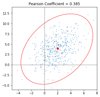
So the mean directly represents the center of the ellipse and the standard deviations provide the boundaries of the rectangle that the ellipse fits into. However, it is not trivial to get the proportions of the ellipse right - its radii, or the relation of the radii, at least. The Pearson Coefficient, however, seems to represent exactly that piece of information: the relation of the radii of the ellipse.
I expect a normalized covariance ellipse to have the following properties:
- Its center should be at the origin of the coordinate system. $\lbrack0,0\rbrack$
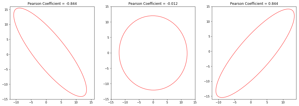
- Since the absolute values of the deviations have been normalized away, the slopes of the axes of our ellipse are 1 and -1 (45° and -45°), respectively.
- Also, the ellipse should fit snugly into a square with a side-length of 2 (normalized deviations from -1 to +1).
- For the extreme values of $p = -1$ and $p = 1$, the length of the non-zero radius is $\sqrt{2}$, because the distance from the origin to any corner of the 2-by-2-square is
When trying to think of a function that might connect the Pearson Coefficient to the radii ($R$) of a normalized ellipse we can start with the following table:
| Pearson | $R$ ascending axis | $R$ descending axis |
|---|---|---|
| -1 | 0.0 | $\sqrt{2}$ |
| 0 | 1.0 | 1.0 |
| 1 | $\sqrt{2}$ | 0.0 |
We can plot these six points like such:
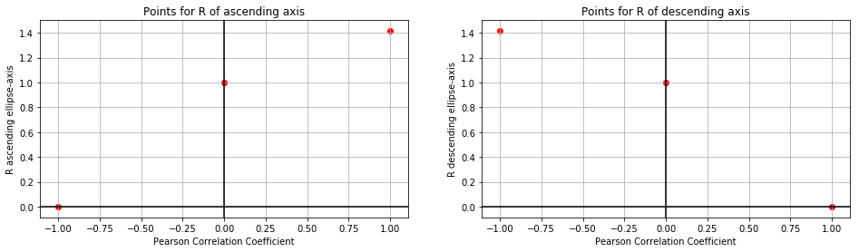
Let’s make a slightly bold assumption: These might be square root functions! With the origin shifted left (and right, respectively):
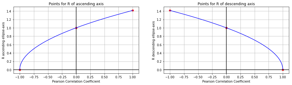
The corresponding functions would be:
\[\text{R ascending axis}=\sqrt{1+p}\] \[\text{R descending axis}=\sqrt{1-p}\]Due to $(-1) <= p <= 1$ it is guaranteed that $(1+p)>=0$ and $(1-p)>=0$ So we will always have an expression $>=0$ under the root.
How it Works: Proof
Now we have had a lot of food for intuition and it is time for the proof.
(I’d also like to show why any ellipse that is calculated like this will always fit snugly into the 2-by-2-square, but this is not an actual proof and I will share this nice fact a little later.)
The proof is where the eigenvalue comes back in. As I mentioned earlier, it is not my idea to get rid of the eigenvalue. I just found a nice way of calculating the eigenvalue for the special case of a normalized 2D covariance ellipse.
The tried and true method to calculate the radii of the covariance ellipse is to choose the radius to be the square root of its corresponding eigenvalue. In the examples I have seen this happens in an un-normalized context, but it works in a normalized context just as well. The only difference is that in a normalized context one standard deviation is always $1$, for all columns. Normalization makes things easier.
So I need to prove that for a normalized dataset with columns x and y the eigenvalues $\lambda_1$ and $\lambda_2$ are
\[\sqrt{\lambda_1}=\sqrt{1+p}\] \[\text{and}\] \[\sqrt{\lambda_2}=\sqrt{1-p}\]Obviously and first of all, we can eliminate the square roots on both sides. (since covariance-matrices are positive semidefinite these eigenvalues can be safely considered to be positive and I already pointed out that $p\pm1>=0$ )
\[\lambda_1=1+p\] \[\lambda_2=1-p\]Then we can grab the math textbook from under our pillow (or wikipedia, for that matter) and look up how we can calculate the eigenvalues of our (2D) normalized covariance matrix.
Often $\mathbf{\Sigma}$ is used to denote a covariance matrix. I will call the normalized covariance matrix $\mathbf{\Sigma_N}$, here. The subscript $N$ stands for “normalized”. $\lambda$ is an eigenvalue of $\mathbf{\Sigma_N}$ and $\mathbf{I}$ is the identity matrix.
\[\begin{vmatrix}\mathbf{\Sigma_N}-\lambda \cdot \mathbf{I}\end{vmatrix}=0\]All $\lambda$s that make the determinant of the difference of the two matrices zero are eigenvalues of $\Sigma_N$.
(In a 2D-case like ours the normalized covariance-matrix is rather straightforward. Note how the variances on the diagonal are both $1$ and how the remaining two positions are occupied by the Pearson Correlation Coefficient.)
\[\begin{align} \begin{vmatrix} \begin{bmatrix} 1 & p \\ p & 1 \end{bmatrix}-\lambda \cdot \begin{bmatrix} 1 & 0 \\ 0 & 1 \end{bmatrix} \end{vmatrix} =0 \end{align}\] \[\begin{align} \begin{vmatrix} 1-\lambda & p \\ p & 1-\lambda \end{vmatrix} =0 \end{align}\] \[\begin{align}(1-\lambda)^2-p^2=0\end{align}\] \[\begin{align}(1-\lambda)^2=p^2\end{align}\]\(\begin{align} 1-\lambda_1=p \text{ and } \lambda_2-1=p \end{align}\) \(\begin{align} \lambda_1=1-p \text{ and } \lambda_2=1+p \end{align}\)
\[q.e.d.\]This way, I have proved, that in fact $1+p$ and $1-p$ are eigenvalues of $\mathbf{\Sigma_N}$.
Since the subscripts for $\lambda$ (“$\lambda_1$” and “$\lambda_2$”) are arbitrary, it should not bother us that the eigenvalues came out to be exactly the other way round.
Still, it would be nice to get a confirmation that these eigenvalues correspond to the axes of the ellipse as I have “guessed”, initially: $1+p$ belonging to the ascending axis and $1-p$ belonging to the descending axis.
I can do this by taking our two eigenvalues and calculating the eigenvectors for them.
Which One Is Which?
Our math textbook says that the relation of eigenvalue and eigenvector is
\[(\mathbf{\Sigma_N}-\lambda_i \cdot \mathbf{I})\cdot \mathbf{v_i} = 0\]$\mathbf{v_i}$ is the eigenvector that is corresponding to the given eigenvalue. $\lambda_i$ is that eigenvalue.
In order to make this operation a lot easier, we can substitute $\lambda_i$ with $1+p$ ($\lambda_1$) and $1-p$ ($\lambda_2$), respectively:
For $\lambda_1= 1+p$ :
\[(\mathbf{\Sigma_N}-(1+p) \cdot \mathbf{I})\cdot \mathbf{v_1} = 0\] \[\left( \begin{bmatrix} 1 & p \\ p & 1 \end{bmatrix}- \begin{bmatrix} 1+p & 0 \\ 0 & 1+p \end{bmatrix} \right) \cdot \mathbf{v_1} =\begin{bmatrix} 0 \\ 0 \end{bmatrix}\] \[\begin{align} \begin{bmatrix} -p & p \\ p & -p \end{bmatrix} \cdot \begin{bmatrix} v_\text{11} \\ v_\text{12} \end{bmatrix} =\begin{bmatrix} 0 \\ 0 \end{bmatrix} \end{align}\] \[\begin{align} \begin{vmatrix} -p\cdot v_\text{11} + p\cdot v_\text{12}=0 \\ p\cdot v_\text{11} -p\cdot v_\text{12}=0 \end{vmatrix} \end{align}\] \[\begin{align} \begin{vmatrix} p\cdot v_\text{12}=p\cdot v_\text{11} \\ p\cdot v_\text{11}=p\cdot v_\text{12} \end{vmatrix} \end{align}\] \[\begin{align} \begin{vmatrix} v_\text{12}=v_\text{11} \\ v_\text{11} = v_\text{12} \end{vmatrix} \end{align}\]The components of the eigenvector $v_1$ that corresponds to the eigenvalue $\lambda_1$ are the same, obviously.
For $\lambda_2= 1-p$ :
\[(\mathbf{\Sigma_N}-(1-p) \cdot \mathbf{I})\cdot \mathbf{v_2} = 0\] \[\left( \begin{bmatrix} 1 & p \\ p & 1 \end{bmatrix}- \begin{bmatrix} 1-p & 0 \\ 0 & 1-p \end{bmatrix} \right) \cdot \mathbf{v_2} =\begin{bmatrix} 0 \\ 0 \end{bmatrix}\] \[\begin{align} \begin{bmatrix} p & p \\ p & p \end{bmatrix} \cdot \begin{bmatrix} v_\text{21} \\ v_\text{22} \end{bmatrix} =\begin{bmatrix} 0 \\ 0 \end{bmatrix} \end{align}\] \[\begin{align} \begin{vmatrix} p\cdot v_\text{21} + p\cdot v_\text{22}=0 \\ p\cdot v_\text{21} + p\cdot v_\text{22}=0 \end{vmatrix} \end{align}\] \[\begin{align} \begin{vmatrix} p\cdot v_\text{21}= -p\cdot v_\text{22} \\ p\cdot v_\text{21}= -p\cdot v_\text{22} \end{vmatrix} \end{align}\] \[\begin{align} \begin{vmatrix} v_\text{21}= -v_\text{22} \\ v_\text{21} = -v_\text{22} \end{vmatrix} \end{align}\]The components of the eigenvector $v_2$ that corresponds to the eigenvalue $\lambda_2$ have the same absolute value but with opposite signs.
Allright! The components of each eigenvector have the same absolute value, and one of them has reversed signs. So the slopes are 1 and -1 (or, again 45° and -45°, respectively). The signs of the eigenvector that comes forth from substituting $(1+p)$ are the same, whereas the signs of the eigenvector that comes forth from substituting $(1-p)$ are reversed. So, in the recipe above, we have correctly assigned $\sqrt{1+p}$ to the ascending axis and $\sqrt{1-p}$ to the descending axis of the covariance ellipse.
Still normalized
That’s all very nice, but it is all still normalized, isn’t it?
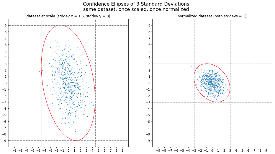
After simplifying the task of getting the right proportions for the confidence ellipse by normalization, we can reverse the consequences of this trick by simply (re-)scaling the normalized and rotated ellipse along the x- and y-axes. More specifically, scaling by the standard deviation of x along the x-axis and scaling by the standard deviation of y along the y-axis.
You can modify these scaling factors by a factor of typically 2 or 3, thus scaling by two or three standard deviations, respectively.
In an earlier version of this post I stated that, according to the 68-95-99.7 rule, 99.7% of the observations of a normally distributed dataset should lie within an ellipse with radiuses of 3 standard deviations. However, I think that I have to correct myself. The 68-95-99.7 rule is valid for a *rectangle* with the dimensions of 2 times 1, 2 or 3 standard deviations. The rule only makes a statement about a one-dimensional dataset and it does not take covariance into account. It is the rectangle that represents this “each dimenson by itself” view of the data. The ellipse, however, follows the bulk of the data more closely and thus “produces” more outliers than you would expect according to the 68-95-99.7 rule. Thanks to colseanm who actually checked my earlier statement.
Summary
In this post I showed an alternative method to produce the confidence ellipse of a covariance just using the means and standarddeviations of the two variables and their mutual covariance. While there are existing methods for this that work just fine, it is nice to know that there is a simple relationship between the Pearson Correlation Coefficient ($p$) and the Eigenvalues of a normalized 2D dataset:
\[\lambda_\text{ascending}=1+p\]and
\[\lambda_\text{descending}=1-p\]Thank you for your attention!
Update
In the meantime, the implementation in the mentioned github-gist has made it into the collection of examples on matplotlib.org.
I have updated the code in the gist according to the example there because thanks to the matplotlib community the code got a lot neater.
Comments
Your feedback and comments are very welcome. Please use the comments function on the gist-page to this post.
(You need to have a gitHub-account, though.)